Fluid flow in a piping system is influenced by several physical and mechanical factors. Understanding these factors helps predict how liquids will behave inside pipes, troubleshoot flow problems, and design systems that operate safely and efficiently. Variables such as viscosity, pipe roughness, velocity, and flow patterns all play a role in determining how easily a liquid moves through a pipe. The following sections explain these factors and how they affect overall system performance.

Viscosity

Viscosity measures a liquid’s internal resistance to flow. It is a form of friction caused by the resistance of fluid molecules moving past one another as they flow through a pipe. In pipe flow, friction is increased by the internal irregularities of the pipe transporting the liquid. Internal bumps and unevenness in a pipe produce a friction force that opposes the liquid flow and slows down its velocity.

If the viscosity is high, the velocity of the liquid is low, and laminar flow occurs, meaning the liquid flows gently in layers through the pipe. A liquid with a low viscosity flows at a higher velocity, and turbulent flow occurs.

Laminar Flow and Turbulent Flow

When a fluid is flowing through a pipe, two types of flow may occur, depending on the velocity of the fluid:

• Laminar flow
• Turbulent flow

Laminar flow, sometimes known as streamline flow, occurs when a fluid flows in parallel layers, with no disruption between the layers. At low velocity, the fluid tends to flow without mixing, and adjacent layers slide past one another like playing cards. There are no cross-currents perpendicular to the direction of flow, nor eddies or swirls of fluids. In laminar flow, the motion of the particles of fluid is very orderly, with all particles moving in straight lines parallel to the pipe walls.

Turbulent flow is the opposite of laminar flow, and occurs at higher velocities, where eddies or cross-currents of fluid particles form, leading to lateral mixing. In non-technical terms, laminar flow is “smooth,” while turbulent flow is “rough.”

Laminar flow, therefore, causes a minimum amount of internal friction between the molecules, and the pressure drop (energy loss) will be relatively small. In comparison, turbulent flow causes a relatively large pressure drop because of the internal resistance caused by fluid particles colliding with each other and the pipe walls.

Ensuring laminar flow is an important consideration at certain points in a piping system. For example, it is especially desirable upstream from metering devices and pressure-regulating valves.

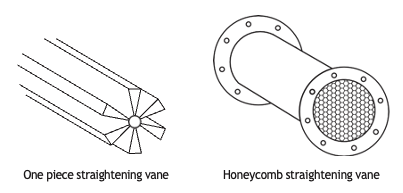
Ordinarily, the flow of fluid through a straight run of unobstructed pipe will be streamline (laminar) if the liquid is not travelling too fast. When the fluid is forced to change direction or an obstruction is encountered, turbulence is created. If it is necessary to install a metering device in a section of pipe where the flow is turbulent, a straightening vane (Figure 1) may be used to provide the streamline (laminar) flow necessary for accurate flow measurement.

Flow Velocity

Velocity describes the speed of motion or flow. It is defined as the rate of motion per unit of time. The common units used to measure velocity of flow are [latex]\frac{\text{ ft.}}{\text{sec.}}[/latex], [latex]\frac{\text{ ft.}}{\text{min.}}[/latex] and [latex]\frac{\text{ m}}{\text{sec.}}[/latex].

In a piping system, the velocity of flow changes when the pipe size changes. When the pipe size is reduced and the volume is constant, the same quantity of liquid must pass through the smaller section of pipe and can only do so by increasing its velocity.

Fluid Velocity and Pressure

Figure 2 shows what happens to pressure when fluid velocity increases.

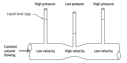
This illustration shows a series of three manometers measuring pressure over a length of pipe in which a liquid is flowing through a graduated venturi (narrowing). This is why pressure drops in narrow sections of pipe. The fluid velocity increases as it passes through the narrower section in order to maintain the same flow rate. At its narrowest point, it reaches its highest velocity and thus lowest flow pressure. Beyond this point, the venturi area increases again. The velocity of the fluid slows down and returns to the entering velocity, while the pressure increases again. A small pressure drop (loss) is observed between the first and third manometer due to friction encountered through the pipe.

Bernoulli’s Principle

Daniel Bernoulli was a Swiss mathematician who pioneered many studies and theories in fluid mechanics. Bernoulli’s principle states that “where velocity is greatest, pressure is least.” This means that as fluid speed increases, pressure decreases.

“Faster flow = lower pressure”

“Slower flow = higher pressure”

Bernoulli’s principle can be derived from the principle of conservation of energy. This states that, in a steady flow, the sum of all forms of energy in a fluid along a pipeline is the same at all points on that pipeline. This requires that the sum of kinetic energy, potential energy and internal energy remains constant. Thus an increase in the speed (velocity) of the fluid—implying an increase in the kinetic energy—occurs with a simultaneous decrease in the sum of the potential energy and internal energy (pressure energy).

Pressure Drop

The loss of pressure, or pressure drop, due to friction as a fluid flows through a piping system may be measured with a gauge or manometer. Pressure drop is often expressed in units of psi, inches of mercury, inches of water column or kPa. The drop in pressure due to friction is also called friction head.

Some of the factors governing the pressure drop due to friction are:

• Viscosity of fluid
• Length of pipe
• Velocity of flow
• Size and type of pipe
• Number and type of fittings and valves
• Number and degree of bends

This pressure drop is observed in the following figure that examines pressure drop due to pipe length. When fluids at rest are in a closed tube, pressure is distributed equally throughout the tube. When the valve is opened and the fluid is allowed to flow, the pressure in the tube will be different at different points along the tube.

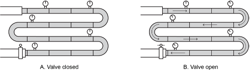
This pressure loss is also affected by material choice. For example, copper pipe typically causes more pressure loss than PVC. Smaller pipe also experiences more pressure drop than larger pipe.

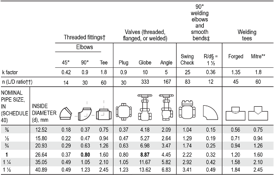
An example of pressure drop due to fittings and valves is found in system design parameters of a natural gas system (Figure 4). In a 1-inch piping system, a 90° elbow has the equivalent pressure drop of 0.80 m of straight sch. 40 steel pipe. Compare this to a 1-inch globe valve that has the equivalent pressure drop of 8.87 m of straight sch. 40 steel pipe.

Self-Test C-1.15: Describe Factors that Affect Fluid Flow in a Piping System

Complete Self-Test C-1.15 and check your answers.

Long Description

Long description of Figure 4 table: Pipe fitting loss coefficients and dimensions

This table presents engineering data used to calculate friction losses in piping systems. It compares different types of pipe fittings and valves by showing their k factors (loss coefficients), equivalent length ratios (L/D), and how these relate to different nominal pipe sizes.

Overall Structure

The table is organized into vertical sections based on fitting type:

1. Threaded fittings (standard): Includes: 45° elbows, 90° elbows, and tees
2. Valves (threaded, flanged, or welded): Includes: plug valves, globe valves, and angle valves
3. 90° welding elbows and smooth bends: Includes: swing check valves and long-radius bends
4. Welding tees: Includes: forged tees and mitre bends

Each category shows:

• A k factor (resistance to flow)
• An n (L/D ratio) representing equivalent pipe length

Top Rows: Flow Resistance Values

k factor (dimensionless)

This row shows how much resistance each fitting adds to fluid flow:

• 45° elbow: 0.42
• 90° elbow: 0.9
• Tee: 1.8
• Plug valve: 0.9
• Globe valve: 10 (very high resistance)
• Angle valve: 5
• Swing check valve: 25 (very high resistance)
• Smooth bend: 0.36 (low resistance)
• Forged tee: 1.35
• Mitre bend: 1.8

Equivalent Length Ratio (n or L/D)

This converts fittings into an equivalent length of straight pipe:

• 45° elbow: 14
• 90° elbow: 30
• Tee: 60
• Plug valve: 30
• Globe valve: 333 (very large equivalent length)
• Angle valve: 167
• Swing check valve: 83
• Smooth bend: 12
• Forged tee: 45
• Mitre bend: 60

Lower Section: Pipe Sizes and Dimensions

The bottom portion lists nominal pipe sizes (Schedule 40) along with their inside diameters in millimetres and metres.

Pipe sizes shown include:

• ⅜ inch (12.52 mm / 0.01252 m)
• ½ inch (15.80 mm / 0.01580 m)
• ¾ inch (20.93 mm / 0.02093 m)
• 1 inch (26.64 mm / 0.02664 m)
• 1¼ inch (35.05 mm / 0.03505 m)
• 1½ inch (40.89 mm / 0.04089 m)

Equivalent Lengths for Each Fitting

For each pipe size, the table shows how much straight pipe length (in metres) each fitting is equivalent to in terms of resistance.

For example:

• A ½-inch pipe:
  • 45° elbow ≈ 0.22 m
  • 90° elbow ≈ 0.47 m
  • Tee ≈ 0.94 m
  • Globe valve ≈ 5.27 m
• A 1-inch pipe:
  • 45° elbow ≈ 0.37 m
  • 90° elbow ≈ 0.80 m
  • Tee ≈ 1.60 m
  • Globe valve ≈ 8.87 m
• A 1½-inch pipe:
  • 45° elbow ≈ 0.49 m
  • 90° elbow ≈ 1.23 m
  • Tee ≈ 2.45 m
  • Globe valve ≈ 13.62 m

Visual Elements

Small line drawings are included above each column to visually represent each fitting type, such as:

• Bent pipe sections for elbows
• T-shaped junctions for tees
• Valve symbols with handles
• Smooth curved bends

Key Takeaway

The table helps users estimate how much resistance different fittings add to a piping system by:

• Comparing fittings using k factors
• Converting them into equivalent pipe lengths
• Adjusting values based on pipe size

This information is commonly used in plumbing and engineering to calculate pressure losses and design efficient piping systems.

References

BCcampus. (n.d.). Playlist: Tools and equipment videos. BCcampus MediaSpace. https://media.bccampus.ca/playlist/details/0_3g8xp22x/categoryId/175673 Playlist Details – Trades Access Common Core Line C: Tools and Equipment Videos – BCcampus

BC Industry Training Authority. (2019). Piping trades apprenticeship program: Use Tools and Equipment—Level 1 harmonized [Binder]. Crown Publications, Queen’s Printer for British Columbia. https://www.crownpub.bc.ca/Product/Details/7960000261_S

• Plumber: Competency C-1 Use Mathematics and Science
• Steamfitter: Competency C-1 Use Mathematics and Science
• Sprinkler Fitter: Competency C-1 Use Mathematics and Science

Camosun College. (2019). Line C: Tools and Equipment—Competency D-2 Apply Science Concepts to Trades Applications (Rev. ed.) [Learning guide]. BCcampus.  https://collection.bccampus.ca/textbook/fkXxtNTn/

Camosun College. (2015). Trades Access Common Core Competency D-2 Apply Science Concepts to Trades Applications. Victoria, B.C.: Crown Publications. Download for free from the B.C. Open Textbook Collection (https://open.bccampus.ca/browse-ourcollection/find-open-textbooks/).

Camosun Innovates. (2022). Tools and Equipment Videos [Video playlist]. Camosun College/BCcampus. https://camosuninnovates.opened.ca/

Flinn, C. (n.d.). OER for Trades: Math for Trades [Video collection]. BCcampus MediaSpace. https://media.bccampus.ca/channel/OER%2Bfor%2BTrades%3A%2BMath%2Bfor%2BTrades/175670
Note: these videos align with the open textbooks Math for Trades: Volume 1 and Math for Trades: Volume 2. All videos are by Chad Flinn and available under a Creative Commons Attribution 4.0 Licence.:

Media Attributions

All figures are sourced from Industry Training Authority (2019) and/or Camosun College (2019) and are used under the Creative Commons Attribution 4.0 (CC BY 4.0) licence unless otherwise noted. Images copyrighted by the BC Industry Training Authority are licensed under a Creative Commons Attribution-NonCommercial-ShareAlike 4.0 (CC BY-NC-SA 4.0) licence.

• Figure 1 Laminar flow  was adapted by TRU Open Press from Dubaj at Wikimedia Commons, and it is in the public domain. Dubaj illustration vectorized by Guillaume Paumier (user:guillom).