Parallel Unequal Spread

Offsets are designed into piping systems when it is necessary for a piping run to avoid an obstacle or another component of the piping system.

When parallel piping runs are installed by a fitter, the pipes run at a certain spread. Spread is the distance (centre-to-centre) between pipes. In many installations, the spread distance changes when we offset around an object. This type of offset is called an unequal spread offset. This piping practice poses aesthetic problems when the piping is exposed, which is common in many industrial applications.

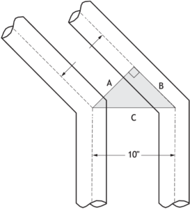
A close look at the start of a 45° offset (Figure 1), shows that the two parallel lines terminate at the same place. This is indicated by the line labelled C. It is also apparent that line C is the hypotenuse of a triangle formed by the shaded area. Once the offset is formed the spread has been reduced by almost 3″ (indicated by line A, which is the adjacent side of the triangle)

Given the original spread of 10″, we can calculate the new spread using trigonometry by solving for the adjacent side:

[latex]\quad\text{cos}(45) \times \text{hypotenuse} = \text{adjacent}[/latex]

Example using 45° elbows:

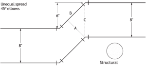
Figure 2 shows a parallel piping run with an 8″ spread. The original route is obstructed by a building column and requires a 6″ offset to go around it using 45° elbows. The original spread (8″) is the hypotenuse of the triangle formed by the dashed lines. The reduced spread through the turn is the adjacent side of the triangle.

Solve for the length of the reduced spread.

Solution:

[latex]\quad\text{cos}(45) \times \text{hypotenuse} = \text{adjacent}[/latex]

[latex]\quad\text{cos}(45) \times 8\text{"} = 5.66\text{"}[/latex]

It is important to note that when the offset terminates, the pipe run returns to its original spread, as shown in Figure 2. The reduced spread (A) is still the adjacent side, and the 8″ spread (C) is the hypotenuse of the triangle.

Example using [latex]22\frac{1}{2}°[/latex] elbows:

Figure 3 shows a parallel piping run with a 10″ spread. The pipe run has a 4″ offset using [latex]22\frac{1}{2}°[/latex] elbows. The original spread (10″) is the hypotenuse of the triangle formed by the dashed lines. The reduced spread, through the turn, is the adjacent side of the triangle.

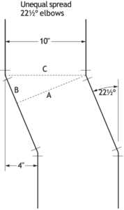
Solve for the length of the reduced spread:

[latex]\quad\text{cos}(22\frac{1}{2}) \times \text{hypotenuse} = \text{adjacent}[/latex]

[latex]\quad\text{cos}(22\frac{1}{2}) \times 10\text{"} = 9.24\text{"}[/latex]

Example using 45° elbows:

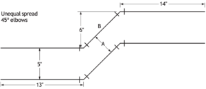
Solve for dimensions A and B in Figure 4.

Solution:

Dimension A:

The original spread is the hypotenuse of the triangle formed by the offset. Dimension A is the reduced spread through the offset, which is the adjacent side of the triangle.

[latex]\quad\text{cos}(45) \times \text{hypotenuse} = \text{adjacent}[/latex]

[latex]\quad\text{cos}(45) \times 5\text{"} = 3.535\text{" or } 3\frac{1}{2}[/latex]

Dimension B:

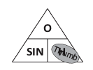
Dimension B is the travel piece length formed by a 6″ offset. Since we are using 45° elbows, the travel will be the hypotenuse of a 6″ triangle. We can solve for this in two ways. One method is to use trigonometry, where the lengths of both the adjacent and opposite sides are 6″, and the length of the hypotenuse is solved using the sin triangle (the sine function on your calculator) (Figure 5).

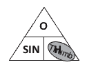
[latex]\quad\frac{6}{\text{sin}(45)} = 8.485 \text{" or }8 \frac{1}{2}\text{"}[/latex]

As mentioned earlier, because we use 45° triangles so often in the piping trades, it is useful to remember the multiplier for a 45° offset. The centre-to-centre length of the travel piece (hypotenuse) will always be 1.414 × the length of either of the shorter sides:

[latex]\quad6\text{"} \times 1.414 = 8.485 \text{" or }8 \frac{1}{2}\text{"}[/latex]

Parallel Equal Spread Offsets

Equal spread offsets are offsets in which the piping’s centre-to-centre measurements remain the same through the offset. This consistent distance is achieved by increasing the length of the pipe on the outside of the offset to maintain equal spacing. This is the preferred way of installing parallel piping runs in our industry.

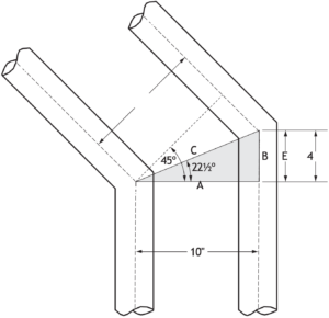
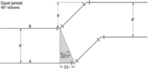
A close look at the 45° offset in Figure 6 shows that the pipes do not start the offset at the same point. The distance that one fitting extends past the next is indicated by the length of line B and is called the extension. If we use the smaller angle as the reference angle, we can see that the known dimension (10″) is the adjacent side, and the extension is the opposite side of the triangle. This reference angle is always half of the fitting angle, in this case [latex]22\frac{1}{2}°[/latex].

Calculating the Extension

As stated earlier, the angle used for calculating the extension for an equal spread offset is half of the fitting angle. This is because the extension is measured from the centre of the fitting, and at that point, only half of the fitting’s deflection has occurred.

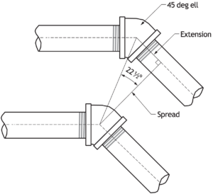
It is important to note that because both the extension and the spread are two sides of the same triangle, when the spread increases, the length of the extension increases proportionally.

To find the length of the extension, we use the given spread (10″) as the adjacent side of the triangle. The length of the extension is the opposite side (B).

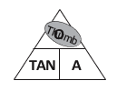
The solution therefore is:

[latex]\quad\text{tan}(22.5) \times 10\text{"} = 4.142\text{"} = 4 \frac{1}{8}\text{"}[/latex]

Example using 45° elbows:

Find the length of the extension for the piping offset in Figure 9, which has an 8″ spread.

Solution:

[latex]\quad\text{tan}(22.5) \times 8\text{"} = 3.314\text{"} = 3 \frac{3}{8}\text{"}[/latex]

Pipe A is longer than pipe B by the length of the extension, in this case, [latex]3\frac{3}{8}\text{"}[/latex].

Example using 60° elbows:

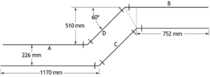
Solve for lengths A, B, C and D in Figure 10.

Solution:

Length A:

Pipe A is shorter than the given dimension (1,170 mm) by the length of the extension formed by a 226-mm spread.

Calculate the extension:

[latex]\quad\text{tan}(30) \times 226 = 130.48\text{ mm}[/latex]

The length of pipe A is:

[latex]\quad1,170 − 130.48 = 1,039.52[/latex]

Length B:

Pipe B is longer than the given dimension (752 mm) by the length of the extension using the same 226-mm spread.

The length of pipe B is:

[latex]\quad752 + 130.48 = 882.48 \text{ mm}[/latex]

Lengths C and D:

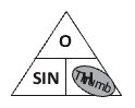
Because these two pipes are parallel and maintain the equal spread, they are of identical length. They are really the hypotenuse of a 60° triangle. The given dimension of 510 mm is the opposite side of the triangle. With this information, sin is the trig function to use (Figure 11).

Solution:

[latex]\quad\frac{510}{\text{sin}(60)} = 588.897 \text{ mm}[/latex]

Self-Test C-1.10.1: Calculate Required Measurements for Piping Offsets

Complete Self-Test C-1.10.1 and check your answers.

Solve for the lengths indicated. Express your answers to the nearest [latex]\frac{1}{8}\text{"}[/latex] or 0.1 mm, as required.

Rolling Offsets

When the travel section in an offset piping arrangement is neither parallel nor perpendicular to the horizontal or vertical planes, the arrangement is called a rolling offset. There are times when both horizontal and vertical direction changes are required to route piping around an obstacle.

The pipe run in Figure 12 shows a typical rolling offset with vertical and horizontal offsets. To visualize the travel of the pipe, imagine a three-dimensional box with the pipe entering at one corner and exiting at the opposite diagonal corner.

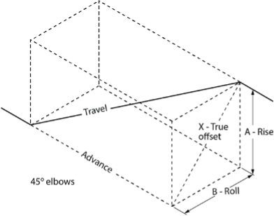
In order to solve for the length of pipe needed for the travel, we must add some dimensions to this imaginary box, starting with the vertical offset dimension, or rise (A), and the horizontal offset dimension, or roll (B). For our example we will use a 30″ vertical rise and 24″ horizontal roll for our offset.

The first step is to find the length of the true offset, which is the diagonal line X in Figure 12.

In past exercises, we found the lengths of different sides of a triangle using trigonometry. When we did this, we knew the reference angle and the length of at least one side. By knowing these two values, we could calculate the lengths of the other two sides.

To solve for the true offset (X), we know the length of two sides, but we do not know the angles (other than one being a right angle). To find the length of the true offset, we must use the Pythagorean theorem.

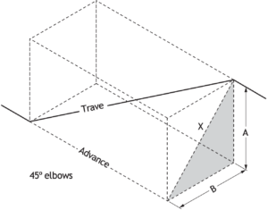
Remember that if we know the lengths of two of the short sides of the shaded triangle, we can solve for the hypotenuse (X) by using the following equation:

[latex]\quad c = \sqrt{a^2 + b^2}[/latex]

In our example, the equation would look like this:

[latex]\quad\text{TO} = \sqrt{30^2 + 24^2}\\ \quad\text{TO} = \sqrt{900 + 576}\\ \quad\text{TO} = \sqrt{1,476}\\ \quad\text{TO} = 38.42\text{"} \space \text{or} \space 38\frac{3}{8}\text{"}[/latex]

Once the true offset has been determined, we can use this measurement to calculate:

• advance (horizontal component)
• travel (actual pipe length)

Referring to Figure 14, we see that the true offset (X) is actually part of two triangles. It serves as the hypotenuse of the dark shaded triangle we solved for earlier using our 30″ and 24″ dimensions. Also, and more importantly, it serves as the opposite side of the light-shaded 45° triangle. This triangle also contains the length of the offset travel (as the hypotenuse) and the length of the offset advance (as side adjacent).

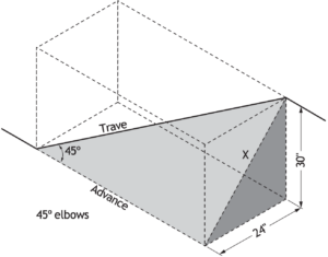
Given the fitting angle, called the reference angle (45), and the length of one side, called side opposite (X), we can now use trigonometry to solve for the two unknown dimensions.

Solve for advance:

Tan is the trig function to use to solve for side adjacent (Figure 15). Using our triangle to solve for the adjacent, the equation should read:

[latex]\quad\frac{\text{opposite}}{\text{tan}(45)} = \text{adjacent}[/latex]

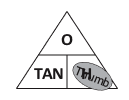
Using the length of the opposite (true offset) as 38.42″, the length of the adjacent would be:

[latex]\quad\frac{38.42}{\text{tan}(45)} = 38.42[/latex]

The lengths of the adjacent and opposite sides are the same in this case. As discussed earlier, this is true for the short sides of all 45° triangles. When solving for other fitting angles ([latex]22\frac{1}{2}°[/latex] or 60°), this will not be the case, and additional trig calculations will need to be used.

Solve for travel:

The travel is the hypotenuse of the 45° triangle and can be found by using the sin function (Figure 16).

[latex]\quad\frac{38.42}{\text{sin}(45)} = 54.33[/latex]

Example:

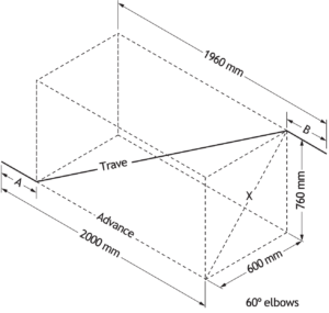
The offset in Figure 17 uses 60° elbows. Solve for the lengths of the following:

a. Solve for true offset:

[latex]\quad\text{TO} = \sqrt{760^2 + 600^2}\\ \quad\text{TO} = \sqrt{577,600 + 360,000}\\ \quad\text{TO} = \sqrt{937,600}\\ \quad\text{TO} = 968.3\text{ mm}[/latex]

b. Solve for advance (adjacent):

[latex]\quad\frac{\text{opposite}}{\text{tan}(60)} = \text{adjacent}\\ \quad\frac{968.3}{\text{tan}(60)} = 559\text{ mm}[/latex]

c. Solve for travel (hypotenuse):

[latex]\quad\frac{\text{opposite}}{\text{sin}(60)} = \text{hypotenuse}\\ \quad\frac{968.3}{\text{sin}(60)} = 1,118.1\text{ mm}[/latex]

d. Solve for dimension A:

[latex]\quad\text{Given Dimension - Advance} = \text{A}\\ \quad2,000 - 559 = 1,441\text{ mm}[/latex]

e. Solve for dimension B:

[latex]\quad\text{Given Dimension - Advance} = \text{B}\\ \quad1,960 - 559 = 1,401\text{ mm}[/latex]

Jumper Offsets

A jumper offset in a piping system uses a combination of fittings to route piping around or over an obstacle such as a duct, column, or other object. Unlike a rolling offset, a jumper offset changes direction in only one plane. There are two common configurations for jumper offsets, both of which contain 45° fittings:

• two 45° elbows and one 90° elbow
• four 45° elbows

This approach provides a more streamlined flow path compared to the installation of four 90° fittings.

The key to solving jumper offsets is recognizing where the 45° triangles occur in the layout.

• Multiply a short side by 1.414 to find the hypotenuse
• Divide the hypotenuse by 1.414 to find a short side

The key to solving for the lengths of a piping arrangement is the ability to recognize where the 45° triangles are located in the offset.

Example 1:

Figure 18 shows a jumper piping offset containing two 45° fittings and one 90° fitting. The piping is installed to ”jump” over a run of circular ductwork.

Solve for the centre-to-centre lengths of the lettered pipe sections indicated using the following information:

• Duct diameter = 8″
• Space between outside of duct and pipe’s centreline = 1″

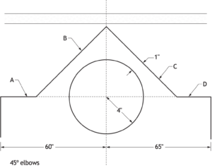
Step 1: First, find the side of the secondary square or right angle triangle. (Figure 19). Scribe a line from centre of the duct rising at 45° until it intersects the centreline of the diagonal pipe B. Once the side of the secondary square is established, you can now find its length:

[latex]\quad\text{duct radius} + \text{space} = \text{length of secondary square}[/latex]

[latex]\quad4\text{"} + 1\text{"} = 5\text{"}[/latex]

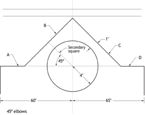
Step 2: Multiplying the secondary square by 2 will give you the lengths of pipes B and C, as both start and end at the centreline of the duct.

Step 3: Finding the length of pipe A will require two steps: first, multiply the length of the secondary square dimension by 1.414 to find the length of the hypotenuse (Figure 20) (this will be the horizontal distance from the centreline of the duct to the centre of the 45° elbow).

[latex]\quad\text{Hypotenuse} = 5\text{"} \times 1.414 = 7.07\text{"}[/latex]

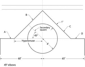
Next, subtract the length of the hypotenuse from the given dimension of 60″:

[latex]\quad\text{A} = (60 − 7.07) = 52.93\text{"}[/latex]

Step 4: The length of pipe D is found using the same procedure used to find the length of pipe A. Multiply the length of secondary square dimension by 1.414 to find the length of the hypotenuse (Figure 21) (this will be the horizontal distance from the centreline of the duct to the centre of the 45° elbow).

[latex]\quad\text{Hypotenuse} = 5\text{"} \times 1.414 = 7.07\text{"}[/latex]

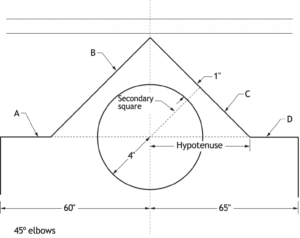
Subtract the length of the hypotenuse from the given dimension of 65″:

[latex]\quad\text{D} = 65 − 7.07 = 57.93\text{"}[/latex]

Example 2:

Solve for the centre-to-centre lengths of the lettered pipe sections indicated in Figure 22 using the following information:

• Duct diameter = 20″
• Space between duct and pipe centre = 2″

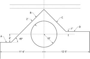
This example is more complex than the previous example, as the horizontal sections of the piping system differ in elevations. The pipe enters the offset 4″ below the centreline of the duct and exits the offset 1″ above the centreline of the duct.

It is important to always use the centreline of the duct as a reference point when establishing triangles used in solving pipe lengths.

Step 1: Find the length of the secondary square side:

[latex]\quad\text{duct radius} + \text{space} = \text{length of secondary square (L)}[/latex].

[latex]\quad10\text{"} + 2\text{"} = 12\text{"}[/latex]

Step 2: Multiply the secondary square by 2 to give you the partial length of pipe B, measured from the peak of the offset to where pipe B intersects the centreline of the duct ([latex]2 \times \text{L}[/latex]).

Pipe B is longer than ([latex]2 \times \text{L}[/latex]) by the length of the hypotenuse formed by the 4″ triangle (seen at H in Figure 23).

[latex]\quad4\text{"} \times 1.414 = 5.656\text{"}[/latex]

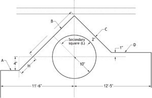
Solve for the length of pipe B:

[latex]\quad\text{B} = (2 \times \text{L}) + \text{H}\\ \quad= (2 \times 12) + 5.656\\ \quad= 24 + 5.656\\ \quad= 29.656\text{" or } 29\frac{5}{8}\text{"}[/latex]

Step 3: To find the length of A, first determine how far the 45° elbow is away from the vertical centreline of the duct.

In Step 1, we determined the length of pipe B, which is really the hypotenuse formed by the dashed lines shown in Figure 24. The distance from the vertical centreline of the duct and the 45° elbow is the short side of that same triangle. To find this dimension, divide the length of pipe B (hypotenuse) by 1.414, which will give us the length of one of the shorter sides:

[latex]\quad\frac{29.656}{1.414} = 20.97\text{"}[/latex]

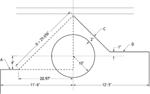
The given dimension of 11′ 6″ is measured from the vertical centreline of the duct to the start of pipe A. Pipe A is measured from the riser to the centre of the 45° elbow. The difference between the given dimension and pipe A would be the short side of the triangle, or 20.97.

[latex]\quad\text{Pipe A} = 11\text{'} 6\text{"} - 20.97\text{"}\\ \quad= 138\text{"} - 20.97\text{"}\\ \quad= 117.03 \text{" or } 117\text{"}[/latex]

Step 4: To find the length of pipe C, first multiply the secondary square by 2; which will give you the length from the peak of the offset to where pipe C would intersect the centreline of the duct ([latex]2 \times \text{L}[/latex]). However, pipe C does not travel to this point but instead levels out 1″ above the horizontal centreline of the duct.

Pipe C is shorter than 2L by the length of the hypotenuse formed by the 1″ triangle (seen at H in Figure 25).

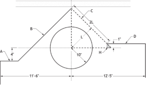
[latex]\quad\text{H} = 1\text{"} \times 1.141 = 1.414\text{"}[/latex]

The length of pipe C is then:

[latex]\quad\text{Pipe C} = 2\text{L} - \text{H}\\ \quad= 24 - 1.414\\ \quad= 22.586 \text{" or } 22\frac{5}{8}\text{"}[/latex]

Step 5: To find the length of D, we must determine how far the 45° elbow is away from the vertical centreline of the duct (Figure 26).

In Step 1, we determined the length of the secondary square to be 12″. If we solved for the hypotenuse of this triangle, it would be 12 × 1.414 = 16.97″. Because the 45° elbow in this question is 1″ closer to the vertical centreline of the duct, the distance from the centreline of the duct to the 45° elbow is now as follows:

[latex]\quad16.97 − 1 = 15.97\text{"}[/latex]

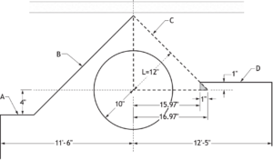
The given dimension of 12′ 5″ is measured from the vertical centreline of the duct to the start of the turn at pipe D. Pipe D is measured from the centre of the riser at the turn to the centre of the 45° elbow. The difference between the given dimension and pipe D would be the hypotenuse of the triangle minus 1″, or 15.97″.

Then:

[latex]\quad\text{Pipe D} = 12\text{'} 5\text{"} - 15.97\text{"}\\ \quad= 149\text{"} - 15.97\text{"}\\ \quad= 125.03\text{" or } 125\text{"}[/latex]

Example 3:

Solve for the centre-to-centre lengths of the lettered pipe sections indicated in Figure 27 using the following information:

• Duct diameter = 10″
• Space between duct and pipe centre = 4″

This pattern of jumper offset uses two 45° elbows at the peak instead of one 90° elbow.

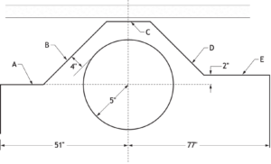
Step 1: As with all jumper offsets, the first thing to find is the side of the secondary square. Scribe a line from the centre of the duct rising at 45° until it intersects the centreline of the diagonal pipe B (Figure 28). Once the side of the secondary square is established, you can find its length:

[latex]\quad\text{Duct radius} + \text{space} = \text{length of secondary square}[/latex]

[latex]\quad5\text{"} + 4\text{"} = 9\text{"}[/latex]

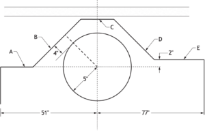
Once you have determined the length of the secondary square, that length will also be the portion of pipe B indicated by the dashed line. This is because the lengths of the short sides of a 45° triangle are always equal.

Step 2: To solve for the length of the short section of pipe B, scribe a line from the centre of the duct to the centre of the upper 45° elbow, as shown in Figure 29. This new line in combination with the secondary square line forms a [latex]22\frac{1}{2}°[/latex] triangle, with the secondary square line becoming the adjacent side and the portion of pipe B in question becoming the opposite side.

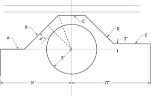
To solve for this portion of pipe B, we will use a trig function that compares the opposite side and the adjacent side. The trig function tan (Figure 30) will be used to solve for the length of the opposite side.

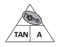
Remember that the adjacent side is the length of the secondary square = 9″:

[latex]\quad\text{opposite} = \text{tan}(22.5) \times \text{adjacent}\\ \quad\text{opposite} = \text{tan}(22.5) \times 9\text{"}\\ \quad\text{opposite} = 3.73\text{"}[/latex]

Therefore, the length of pipe B is the opposite side of the [latex]22\frac{1}{2}°[/latex] triangle plus the length of the secondary square:

[latex]\quad\text{Pipe B} = 9 + 3.73 = 12.73\text{"}[/latex]

Step 3: As before, in order to find the length of A, we must determine how far the lower 45° elbow is away from the vertical centreline of the duct.

In Step 1, we determined the length of the secondary square, which is the length of a short side of the triangle, represented by dashed lines in Figure 31. The distance from the vertical centreline of the duct to the 45° elbow is the hypotenuse of that same triangle. To find this dimension, we simply multiply the length of the secondary square by 1.414, which will give us the length of the hypotenuse.

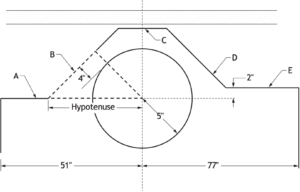
The length of the hypotenuse is then:

[latex]\quad9\text{"} \times 1.414 = 12.73\text{"}[/latex]

The given dimension of 51″ is measured from the vertical centreline of the duct to the start of pipe A. Pipe A is measured from the riser to the centre of the 45° elbow. The difference between the given dimension and pipe A would be the hypotenuse of the triangle, or 12.37. The length of pipe A is therefore:

[latex]\quad\text{Pipe A} = 51 - 12.37\\ \quad= 38.63\text{" or } 38\frac{5}{8}\text{"}\\[/latex]

Step 4: Recall a calculation in Step 2, where trig was used to solve for the opposite side of a [latex]22\frac{1}{2}°[/latex] triangle that made up a portion of pipe B. The resulting length of this portion was 3.73″. If lines are scribed as shown in Figure 32, you can see that four identical [latex]22\frac{1}{2}°[/latex] triangles are formed.

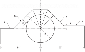
The length of line C is the sum of two of these opposite sides, and thus:

[latex]\quad\text{Pipe C} = 2 \times 3.73\\ \quad= 7.46\text{"}\\[/latex]

Step 5: To solve for the length of pipe D, you can see from Figure 33 that there are three component lengths to consider, indicated by the dashed lines:

1. The opposite side of a [latex]22\frac{1}{2}°[/latex] triangle, previously calculated to equal 3.73″
2. The short side of a secondary square 45° triangle, previously calculated to be 9″
3. The hypotenuse of a 2″ triangle created when the pipe offset exited before reaching the duct centreline:

[latex]\quad2 \times 1.414 = 2.828\text{"}[/latex]

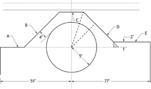
The length of pipe D is then:

[latex]\quad\text{Pipe D} = 3.73 + 9 - 2.828\text{"}\\ \quad= 9.9\text{"}\\[/latex]

Step 5: Similar to the previous example, to find the length of E, we must determine how far the 45° elbow is away from the vertical centreline of the duct (Figure 34).

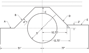
To find the length of E, we must determine how far the 45° elbow is away from the vertical centreline of the duct. In Step 1 we determined the length of the secondary square to be 9″. If we solved for the hypotenuse of this triangle, it would be [latex]9\text{"} \times 1.414 = 12.73\text{"}[/latex]. Because the 45° elbow in question is 2″ closer to the vertical centreline of the duct, the distance from the centreline of the duct to the 45° elbow is now:

[latex]\quad12.73 − 2 = 10.73\text{"}[/latex]

The given dimension of 77″ is measured from the vertical centreline of the duct to the start of pipe E. Pipe E is measured from the riser to the centre of the 45° elbow. The difference between the given dimension and pipe E would be the hypotenuse of the triangle minus 2″, or 10.73″.

Then:

[latex]\quad\text{Pipe E} = 77\text{"} - 10.73\text{"}\\ \quad= 77\text{"} - 10.73\text{"}\\ \quad= 66.27\text{, or } 66\frac{1}{4}\text{"}[/latex]

Self-Test C-1.10.2: Calculate Required Measurements for Piping Offsets

Complete Self-Test C-1.10.2 and check your answers.

Solve for the lengths indicated. Express your answers to the nearest [latex]\frac{1}{8}\text{"}[/latex] or [latex]\frac{1}{10}\text{ mm}[/latex], as required.

References

BCcampus. (n.d.). Playlist: Tools and equipment videos. BCcampus MediaSpace. https://media.bccampus.ca/playlist/details/0_3g8xp22x/categoryId/175673 Playlist Details – Trades Access Common Core Line C: Tools and Equipment Videos – BCcampus

BC Industry Training Authority. (2019). Piping trades apprenticeship program: Use Tools and Equipment—Level 1 harmonized [Binder]. Crown Publications, Queen’s Printer for British Columbia. https://www.crownpub.bc.ca/Product/Details/7960000261_S

• Plumber: Competency C-1 Use Mathematics and Science
• Steamfitter: Competency C-1 Use Mathematics and Science
• Sprinkler Fitter: Competency C-1 Use Mathematics and Science

Camosun College. (2019). Line C: Tools and Equipment—Competency D-1: Solve Trades Mathematical Problems (Rev. ed.) [Learning guide]. BCcampus.  https://collection.bccampus.ca/textbook/qFKGAJ78/

Camosun College. (2015). Trades Access Common Core Competency D-1: Solve Trades Mathematical Problems. Victoria, B.C.: Crown Publications. Download for free from the B.C. Open Textbook Collection (https://open.bccampus.ca/browse-ourcollection/find-open-textbooks/).

Camosun Innovates. (2022). Tools and Equipment Videos [Video playlist]. Camosun College/BCcampus. https://camosuninnovates.opened.ca/

Flinn, C. (n.d.). OER for Trades: Math for Trades [Video collection]. BCcampus MediaSpace. https://media.bccampus.ca/channel/OER%2Bfor%2BTrades%3A%2BMath%2Bfor%2BTrades/175670
Note: these videos align with the open textbooks Math for Trades: Volume 1 and Math for Trades: Volume 2. All videos are by Chad Flinn and available under a Creative Commons Attribution 4.0 Licence.:

Media Attributions

All figures are sourced from Industry Training Authority (2019) and/or Camosun College (2019) and are used under the Creative Commons Attribution 4.0 (CC BY 4.0) licence unless otherwise noted. Images copyrighted by the BC Industry Training Authority are licensed under a Creative Commons Attribution-NonCommercial-ShareAlike 4.0 (CC BY-NC-SA 4.0) licence.